Machine Learning (ML) represents a departure from traditional rule-based programming by allowing systems to learn from data. While the latter requires explicit rules and structures, ML algorithms can uncover patterns and make decisions or predictions autonomously.

Core Distinctions

1. Input-Output Mechanism:

   • Traditional Programming: Takes known input, applies rules, and produces deterministic output.
   • Machine Learning: Learns mappings from example data, generalizing to make predictions for unseen inputs.

2. Human Involvement:

   • Traditional Programming: Rule creation and feature engineering often require human domain knowledge.
   • Machine Learning: Automated model training reduces the need for explicit rules, although human insight is still valuable in data curation and algorithm selection.

3. Adaptability:

   • Traditional Programming: Changes in underlying patterns or rules necessitate code modification.
   • Machine Learning: Models can adapt to some changes, but continuous monitoring is required, and adaptation isn’t always instantaneous.

4. Transparency:

   • Traditional Programming: Generally has explainable, rule-based logic.
   • Machine Learning: Some algorithms might be “black boxes,” making it challenging to interpret the reasoning behind specific predictions.

5. Applicability:

   • Traditional Programming: Well-suited for tasks with clear, predefined rules.
   • Machine Learning: Effective when facing complex problems with abundant data, such as natural language processing or image recognition.

Code Example: “Hello, World!” Programs

Here are the Python code snippets.

Traditional Programming:

def hello_world():
    return "Hello, World!"

print(hello_world())

Machine Learning:

# Import the relevant library
from sklearn.linear_model import LinearRegression
import numpy as np

# Prepare the data
X = np.array([1, 2, 3, 4, 5]).reshape(-1, 1)
y = np.array([2, 3, 4, 5, 6])

# Instantiate the model
model = LinearRegression()

# Train the model (in this case, it's just fitting the data)
model.fit(X, y)

# Make a prediction function
def ml_hello_world(x):
    return model.predict(x)

# Test the ML prediction
print(ml_hello_world([[6]]))  # Output: [7.]

Supervised and unsupervised learning are fundamental paradigms in the realm of machine learning, each with its unique approach to handling data.

Supervised Learning

In supervised learning, the algorithm learns from a labeled dataset, where the inputs (features) and the correct outputs (labels) are provided. The goal is to build a model that can make accurate predictions or classifications for unseen data.

Key Characteristics:

• Training with Labels: The algorithm is trained on labeled data, allowing it to learn the relationship between inputs and outputs.
• Performance Evaluation: The model’s predictions are evaluated against the true labels in the training data.
• Tasks: Well-defined tasks such as classification (e.g., spam detection) or regression (e.g., predicting house prices) are common.

Unsupervised Learning

In contrast to supervised learning, unsupervised learning doesn’t rely on labeled data for training. Instead, it focuses on discovering underlying patterns or structures within the data.

Key Characteristics:

• Training without Labels: The algorithm processes unlabeled data, thereby learning structure and patterns inherent to the data itself.
• Performance Evaluation: Since there are no labels, evaluation is often more subjective or based on specific application goals.
• Tasks: Unsupervised methods are often used for data exploration, clustering (grouping similar data points) and dimensionality reduction.

Hybrid Approaches

There also exist learning paradigms that blend aspects of both supervised and unsupervised learning. This approach is known as semi-supervised learning and is particularly useful when labeled data is scarce or expensive to obtain.

Feature selection plays a crucial role in machine learning, streamlining models for improved performance, interpretability, and efficiency.

Key Considerations

1. Dimensionality Reduction: High-dimensional data can lead to overfitting and computational challenges. Selecting relevant features can mitigate these issues.

2. Model Performance: Extraneous features can introduce noise or redundant information, compromising a model’s predictive power.

3. Interpretability: Selecting a subset of the most important features can often make a model more understandable, especially for non-black box models.

4. Computational Efficiency: Used reduced feature sets can speed up training and prediction times.

Feature Selection Methods

Filter Methods

These methods preprocess data before model building:

• Variance Threshold: Remove low-variance features that offer little discriminatory information.
• Correlation Analysis: Remove one of two highly correlated features to address redundancy.
• Chi-Squared Test: Rank and select features based on their association with the target variable in classification tasks.

Wrapper Methods

These methods evaluate models with different feature subsets, often using a cross-validation strategy:

• Forward Selection: Starts with an empty set and adds features one at a time based on model performance metrics.
• Backward Elimination: Starts with all features and removes them one by one, again based on performance metrics.
• Recursive Feature Elimination (RFE): Uses models like logistic regression that assign weights to features, and eliminates the least important features.

Embedded Methods

These methods incorporate feature selection directly into the model training process:

• Lasso (L1 Regularization): Adds a penalty equivalent to the absolute value of the magnitude of the coefficients, leading to feature selection.
• Tree-Based Selection: Decision trees and their ensembles (e.g., Random Forest, Gradient Boosting Machines) naturally assign feature importances, which can be used for selection.
• Feature Importance from Model Algorithms: Some models, like Random Forest or LightGBM, provide metrics on feature importance, which can be used to select the most relevant features.

Overfitting and underfitting are phenomena that arise when training machine learning models.

Overfitting

Overfitting occurs when a model learns the training data too well. As a result, it performs poorly on unseen (test or validation) data. Symptoms of overfitting include high accuracy on the training data but significantly lower accuracy on test data.

This is akin to “memorization” rather than learning from the data’s inherent patterns. Reasons for overfitting include the model being too complex or the training data being insufficient or noisy.

Visual Representation

When you look at a graph, you will notice that the “model’s line wiggles a lot” to try and accommodate most of the data points.

Underfitting

Underfitting happens when a model performs poorly on both the training data and the test data. This occurs because the model is too simple to capture the underlying patterns of the data.

In essence, the model “fails to learn” from the training data. Causes of underfitting often stem from using overly simplistic models for the data at hand or from having an inadequate amount of training data.

Visual Representation

The “model’s line” will be a simple one (like a straight line for linear models) that misses a lot of the data’s intricacies.

Ideal Fitting

The goal in machine learning is to achieve optimal generalization, where a model performs well on both seen and unseen data. This balancing act between overfitting and underfitting is termed “ideal fitting”.

A model that achieves ideal fitting has learned the underlying patterns in the data without memorizing noise or being so inflexible as to miss important trends.

Visual Representation

The “model’s line” follows the data points closely without overemphasizing noise or missing key patterns.

Strategies to Counter Overfitting

1. Simplify the Model: Use a simpler model, such as switching from a complex deep learning architecture to a basic decision tree.
2. Feature Selection: Choose only the most relevant features and discard noisy or redundant ones.
3. Regularization: Add penalties for large coefficients, as in Lasso or Ridge regression.
4. Cross-Validation: Use more of the available data for both training and testing, especially in smaller datasets.
5. Early Stopping: Halt the training process of models like neural networks as soon as the performance on a validation set starts to degrade.

Code Example: Decision Tree with Limited Depth

Here is the Python code:

from sklearn.tree import DecisionTreeClassifier

# Limiting tree depth to 3
dt = DecisionTreeClassifier(max_depth=3)

Strategies to Counter Underfitting

1. Increase Model Complexity: Use more advanced models that can capture intricate patterns.
2. Feature Engineering: Derive new, more informative features from the existing ones.
3. More Data: Especially for complex tasks, having a larger dataset can help the model understand underlying patterns better.
4. Hyperparameter Tuning: Adjust the settings of the learning algorithm or model to get the best performance.
5. Ensemble Methods: Combine predictions from multiple models to improve overall performance.

Cross-validation is a robust method for estimating the performance of a machine learning model. Its key advantage over a simple train/test split is that it uses the full dataset for both training and testing, resulting in a more reliable performance metric.

Why Use Cross-Validation Over Train/Test Split?

• Maximizes Dataset Utility: With cross-validation, every data point is used for both training and testing, minimizing information loss.
• More Reliable Performance Estimates: Cross-validation produces multiple performance metrics (such as accuracy or mean squared error), allowing for the calculation of standard deviation and confidence intervals.
• Helps Combat Overfitting: Models consistently performing better on the training set than the test set are likely overfitted, a phenomenon easily detectable with cross-validation.

Common Types of Cross-Validation

1. k-Fold Cross-Validation: The dataset is divided into $k$ roughly equal-sized folds. The model is trained $k$ times, each time using $k-1$ folds as the training set and the remaining fold as the test set.
2. Leave-One-Out Cross-Validation (LOOCV): A special case of k-fold cross-validation where $k$ equals the number of instances in the dataset. Each individual data point is used as the test set, with the remaining data points used for training.
3. Stratified Cross-Validation: Ensures that each fold maintains the same class distribution as the original dataset. This is especially useful for imbalanced datasets.

Code Example: k-Fold Cross-Validation

Here is the Python code:

import numpy as np
from sklearn.model_selection import cross_val_score, KFold
from sklearn.linear_model import LogisticRegression
from sklearn.datasets import load_iris

# Load the Iris dataset
X, y = load_iris(return_X_y=True)

# Create a k-Fold cross-validation splitter
kfold = KFold(n_splits=5, shuffle=True, random_state=42)

# Initialize a classifier
classifier = LogisticRegression()

# Perform k-Fold cross-validation
cv_scores = cross_val_score(classifier, X, y, cv=kfold)
print("Cross-validated accuracy scores:", cv_scores)
print("Mean accuracy:", np.mean(cv_scores))

The Bias-Variance Tradeoff is a fundamental concept in machine learning that deals with the interplay between a model’s complexity, its predictive performance, and its generalizability to unseen data.

Sources of Error

When a machine learning model makes predictions, there are several sources of error:

1. Bias (Systematic Error): Arises when a model is consistently inaccurate, typically due to oversimplified assumptions.
2. Variance (Random Error): Reflects the model’s sensitivity to the training data; a high-variance model can overfit and capture noise.

The tradeoff stems from the fact that as you try to reduce one type of error, the other may increase.

Visual Representation

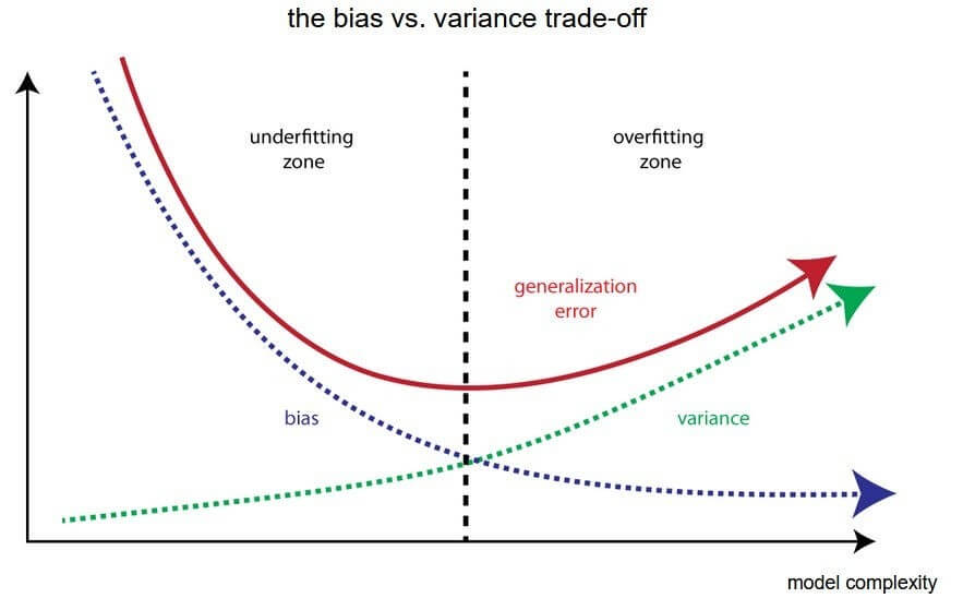
Overfitting and Underfitting

• Overfitting: High model complexity fits the training data too closely and performs poorly on unseen data (high variance).
• Underfitting: The model is too simple to capture the underlying patterns in the data and thus has poor performance on both the training and test data (high bias).

Desired Model Sweet Spot

Aim for a model that generalizes well to new, unseen data:

• Generalization: A model that strikes a good balance between bias and variance will be more robust and have better predictive performance on unseen data.
• Simplicity: Whenever possible, it’s advisable to choose a simpler model that generalizes well.

Strategies to Navigate the Tradeoff

• Cross-Validation: Helps in estimating the model’s performance on new data.
• Learning Curves: Plotting training and validation scores against the size of the training set can provide insights.
• Regularization: Techniques like Lasso or Ridge can help control model complexity.

Code Example: Decision Tree Classifier

Here is the Python code:

import numpy as np
import matplotlib.pyplot as plt
from sklearn.model_selection import learning_curve
from sklearn.tree import DecisionTreeClassifier

# Generate sample data
np.random.seed(0)
X = np.random.rand(100, 1)
y = np.cos(2.5 * np.pi * X).ravel()

# Instantiate a decision tree classifier
dt = DecisionTreeClassifier()

# Compute learning curve scores
train_sizes, train_scores, valid_scores = learning_curve(dt, X, y, train_sizes=np.linspace(0.1, 1.0, 10))

# Plot learning curve
plt.plot(train_sizes, np.mean(train_scores, axis=1), label='Training Score')
plt.plot(train_sizes, np.mean(valid_scores, axis=1), label='Validation Score')
plt.xlabel('Training Samples')
plt.ylabel('Score')
plt.title('Learning Curve')
plt.legend()
plt.show()

Regularization is a set of techniques used in machine learning to prevent overfitting. It accomplishes this by adding penalties to the model’s loss function, leading to more generalized models. Two common types of regularization are Lasso (L1) and Ridge (L2), each with its unique penalty strategy.

L1 and L2 Regularization

• L1 regularization adds a penalty proportional to the absolute values of the coefficients. This can lead to sparse models where less important features have a coefficient of zero.

• L2 regularization squares the coefficients and is known for its tendency to distribute the coefficient values more evenly.

Techniques to Prevent Overfitting

1. Early Stopping: Training is halted when the model’s performance on a validation dataset starts to degrade.

2. Cross-Validation: The dataset is divided into subsets, and the model is trained and validated multiple times, allowing a more robust evaluation.

3. Ensemble Methods: Techniques like bagging and boosting train multiple models and combine their predictions to reduce overfitting.

4. Pruning: Commonly used in decision trees, it involves removing sections of the tree that provide little predictive power.

5. Feature Selection: Choosing only the most relevant features for the model can reduce the chance of overfitting.

6. Data Augmentation: Introducing variations of the existing data can help prevent the model from learning the training data too well.

7. Simpler Algorithms: In some cases, using a less complex model can be more effective, especially when the data is limited.

In statistical modeling, there is a distinction between parametric and non-parametric methods, each with unique strengths and limitations.

Parametric Models

Parametric models make specific assumptions about the data distribution from which the sample is drawn. Once these assumptions are met, parametric models typically offer increased efficiency with simpler and faster computations.

Common parametric models include:

• Linear Regression: Assumes a linear relationship between variables and normal distribution of errors.
• Logistic Regression: Assumes a linear relationship between variables and that errors are independent and follow a binomial distribution.
• Normal Distributions-Based Methods (t-tests, ANOVA): Assume data is normally distributed.

Non-Parametric Models

Non-parametric models, in contrast, make fewer distributional assumptions. They are often more flexible and can be applied in a wider range of situations, at the cost of requiring more data for accurate estimations.

Common non-parametric models include:

• Decision Trees: Segments data into smaller sets, making no distributional assumptions.
• Random Forest: An ensemble method often used for classification and regression tasks that averages multiple decision trees.
• K-Nearest Neighbors: Makes predictions based on similarities to other data points.
• Support Vector Machines (SVM): Effective for classification tasks and doesn’t make strong assumptions about the distribution of the input data.

Hybrid and Semiparametric Models

There is also a middle ground between the parametric and non-parametric extremes. Semiparametric methods combine some of the parametric and non-parametric advantages.

For example, the Cox Proportional Hazards model used in survival analysis combines a parametric model for the baseline hazard (logistic or normal, typically) with a non-parametric model for the effect of the predictors.

Other hybrid models, like the Generalized Additive Model (GAM), introduce non-linear relationships in a parametric framework, offering greater flexibility than purely parametric methods but often with more interpretability than non-parametric approaches.

The curse of dimensionality is a phenomenon that arises when working with high-dimensional data, leading to significant challenges in problem-solving, computational efficiency, and generalization for machine learning algorithms.

Key Challenges Arising from High Dimensions

1. Increased Sparsity: As the number of dimensions grows, the volume of the sample space expands rapidly, resulting in sparser data. This may lead to a scarcity of data points, making it difficult for algorithms to identify meaningful patterns or relationships.

2. Data Overfitting: High-dimensional spaces offer more opportunities for chance correlations. Consequently, an algorithm trained on such data is more likely to fit the noise in the dataset, leading to poor performance on unseen data.

3. Computational Hurdles: Many machine learning techniques exhibit an exponential growth in computational requirements as the number of dimensions increases. This can make analysis infeasible or lead to a reliance on limited approximations.

4. Data Redundancy: Paradoxically, while high-dimensional spaces can be sparse, they can also exhibit redundancy. This means that even with a large number of dimensions, some of the information in the data could be duplicated or highly correlated.

5. Feature Selection and Interpretability: In high-dimensional settings, identifying the most relevant features can be challenging. Moreover, as the number of dimensions grows, so does the difficulty of interpreting and understanding the relationships within the data.

6. Increased Sample Size Requirements: To maintain a certain level of statistical confidence in high-dimensional spaces, the required sample size often needs to grow exponentially with the number of dimensions.

Code Example: Curse of Dimensionality Demonstrated with Exponential Growth

Here is the Python code:

import numpy as np
import matplotlib.pyplot as plt

# Range of dimensions
dimensions = np.arange(1, 101)

# Number of points for each dimension
num_points = 10

# Compute and visualize the growth rate
mean_distances = [np.mean(np.linalg.norm(np.random.rand(num_points, dim), axis=1)) for dim in dimensions]

plt.plot(dimensions, mean_distances)
plt.title('Exponential Growth in Sample Space Volume')
plt.yscale('log')
plt.show()

Model complexity refers to how intricate or flexible a machine learning model is in capturing relationships in data. This complexity comes with both advantages and disadvantages in terms of predictive performance and generalizability.

Overfitting: The Pitfall of Over-Complex Models

• Overfitting happens when a model is excessively complex, capturing noise and small fluctuations in the training data that don’t reflect the true underlying patterns. As a result, the model doesn’t generalize well to new, unseen data.

  This can be compared to a student who has memorized the training dataset without understanding the concepts, and then performs poorly on a test that has new questions.

Model Complexity Metrics

Cross-Validation

• K-Fold Cross-Validation: The data is split into K folds; each fold is used as a validation set, and the process is repeated K times, providing an average performance measure.

Learning Curves

• Train-Test Learning Curves: Plots of model performance on the training and test sets as a function of the dataset size can indicate overfitting if the training performance remains high while the test performance plateaus or decreases.

Information Criteria

• AIC and BIC: These metrics, derived from likelihood theory, penalize the number of model parameters. AIC puts a higher penalty, making it more sensitive to overfitting.

Regularization Path

• For models like Lasso and Ridge regression that introduce penalties for model parameters, one can look at how the optimal penalty changes with the strength of regularization.

Balancing Act: Bias vs. Variance

• Bias is the difference between the expected model predictions and the true values.
• Variance is the model’s sensitivity to small fluctuations in the training data.

High model complexity typically leads to low bias but high variance. The challenge is to find a middle ground that minimizes both.

Code Example: AIC and BIC in R

Here is the R code:

# Fit a linear model
model <- lm(Sepal.Length ~ ., data = iris)

# Calculate AIC and BIC
AIC(model)
BIC(model)

Data preprocessing is a crucial step in machine learning that focuses on cleaning, transforming, and preparing raw data for modeling. High-quality inputs are essential for accurate and reliable outputs.

Key Steps in Data Preprocessing

1. Data Cleaning:

   • Identify and handle missing data.
   • Remove duplicate records.
   • Detect and deal with outliers.

2. Data Integration:

   • Merge data from multiple sources.

3. Data Transformation:

   • Convert data to appropriate formats (e.g., categorical to numerical).
   • Normalize data to a standard scale.
   • Discretize continuous attributes.
   • Reduce dimensionality.

4. Data Reduction:

   • Reduce noise in the data.
   • Eliminate redundant features.
   • Eliminate correlated features to avoid multicollinearity.

5. Data Discretization:

   • Binning or bucketing numerical variables.
   • Converting categorical data to numerical form.

6. Feature Engineering:

   • Create new features that capture relevant information from the original dataset.
   • Feature scaling to ensure all features have equal importance.

7. Feature Selection:

   • Identify the most relevant features for the model.
   • Eliminate less important or redundant features.

8. Resampling:

   • Handle imbalanced classes in the target variable.

Code Example: Handling Missing Data

Here is the Python code:

import pandas as pd

# Create a sample DataFrame with missing data
data = {'A': [1, 2, None, 4, 5],
        'B': ['a', 'b', None, 'c', 'a']}
df = pd.DataFrame(data)

# Identify and count missing values
print(df.isnull().sum())

# Handle missing data (e.g., using mean imputation)
mean_A = df['A'].mean()
df['A'].fillna(mean_A, inplace=True)

# Alternatively, you can drop missing rows:
# df.dropna(inplace=True)

Handling missing data is a critical part of data analysis. It ensures the accuracy and reliability of analytical results. Let’s look at different strategies to deal with missing data.

Techniques for Handling Missing Data

1. Deletion

• Listwise Deletion: Eliminates entire rows with any missing values. This method is straightforward but can lead to a significant loss of data.

• Pairwise Deletion: Analyzes data on a pairwise basis, ignoring missing values. While it preserves more data, the sample sizes for specific comparisons may vary, leading to potential inconsistencies.

• Column (Feature) Deletion: Removes entire columns with any missing values. This approach is suitable when only a small proportion of values are missing.

2. Data Imputation

• Mean/Median/Mode: Replace missing values with the mean (for normally distributed data), median, or mode of the column. It’s a simple method but can distort relationships and variability.
• Last Observation Carried Forward (LOCF): Common in time series data, it replaces missing values with the most recent non-missing value.
• Linear Interpolation: Estimates missing values based on a line connecting the two closest non-missing values before and after.
• Regression: Predict missing values using other related variables as predictors. It’s a more complex imputation method.
• K-Nearest Neighbors (KNN): Predict missing values based on the values of the nearest neighbors in the feature space.
• Multiple Imputation: Creates several imputed datasets and analyzes them separately before combining the results. It accounts for the uncertainty associated with imputation.

3. Handling During Data Collection

• Standardized Entry Forms: Ensures all necessary fields are filled out.
• Mandatory Fields: Requires specific fields to be completed.
• Database Constraints: Using constraints like “NOT NULL” can prevent missing data at the system level.

4. Advanced Techniques

• Utilize Algorithms: Some machine learning models handle missing data more gracefully, like Random Forests or XGBoost.
• Predictive Models: Building models to predict missing values using non-missing data as features.
• Domain Knowledge: Understanding the reasons behind missing data and making informed decisions based on that knowledge.

Feature scaling is a crucial data preprocessing step for many machine learning algorithms. It standardizes the range of independent variables, ensuring they contribute to model training in a balanced way.

Why Feature Scaling is Necessary

• Gradient Descent: Many algorithms, such as linear regression, use gradient descent to optimize model parameters. Consistent feature ranges help the algorithm converge more efficiently.

• Distance-Based Metrics: Algorithms like K-Nearest Neighbors are sensitive to feature magnitudes and can yield biased results without scaling.

• Model Interpretability: Coefficients in models like logistic regression reflect feature importance relative to one another. Scaled features provide more meaningful coefficients.

• Equal Algorithm Attention: Unscaled features might dominate the model’s learning process simply because of their larger magnitudes.

Common Scaling Techniques

Min-Max Scaling

• Range: Maps feature values to a range between 0 and 1.
• Use Case: When feature values are uniformly distributed.

Standardization

• Z-Score: Transforms the data to have a mean of 0 and a standard deviation of 1.
• Range: Suitable when data follows a normal distribution.
• Note: Outliers can heavily influence the mean and standard deviation, making this method sensitive to outliers.

Robust Scaling

• Outlier Robustness: Reduces the influence of outliers on the scaled values.
• Use Case: When the dataset contains outliers.

Unit Vector Scaling

• Scale: Transforms the values to have a norm of 1, turning them into vectors on the unit hypersphere.
• Use Case: When only the direction of the data matters, not its magnitude.

Log and Yeo-Johnson Transformations

• Normalization: Useful for features that do not follow a Gaussian distribution.
• Transformation: Maps data to a more normally distributed space.

Mean Normalization

• Adjustment for Mean: Scales the data by subtracting the mean and then dividing by the range.
• Range: Slightly expands the feature space around zero.

Both normalization and standardization are techniques used in data preprocessing to bring the data into a specific range. While they share a similar objective, they employ different statistical methods to achieve it.

Normalization

• Min-Max Scaling: Transforms the data to a given range, typically between 0 and 1, using the formula:

$$\text{X}$${\text{normalized}} = \frac{\text{X} - \text{X}{\text{min}}}{\text{X}{\text{max}} - \text{X}{\text{min}}}

• L2-Norm: Scales the data so that the squared sum of each row or column is 1.

• L1-Norm: Scales the data so that the sum of the absolute values of each row or column is 1.

Standardization

Also known as Z-score Normalization, standardization transforms the data to have a mean of 0 and a standard deviation of 1, using the formula:

$$\text{X}_{\text{standardized}} = \frac{\text{X} - \mu}{\sigma}$$

Here, $\mu$ represents the mean of the feature and $\sigma$ is the standard deviation. Standardization is robust to outliers and preserves useful information about the variance and covariance in the data, making it a common choice, especially for algorithms that rely on the Gaussian distribution, such as Linear Discriminant Analysis (LDA) and Logistic Regression. In contrast, Min-Max Scaling is more appropriate for algorithms like Neural Networks or models where the data should have a specific bounded range.

One-Hot Encoding is a technique often employed with categorical data to make it compatible for machine learning algorithms that expect numerical input.

How it Works

Say you have a feature like “Color” with three categories: Red, Green, and Blue. You’d create three binary columns – one for each color – where a 1 indicates the presence of that color and 0s the absence.

Red	Green	Blue
1	0	0
0	1	0
0	0	1

In this way, you convert each categorical entry into a binary vector.

Code Example: One-Hot Encoding

Here is the Python code:

import pandas as pd

# Sample data
data = {'Color': ['Red', 'Green', 'Blue', 'Blue', 'Red']}
df = pd.DataFrame(data)

# One-hot encoding
one_hot_encoded = pd.get_dummies(df, columns=['Color'])
print(one_hot_encoded)

Advantages

• Algorithm Compatibility: Most ML algorithms work better with numerical data.
• Category Preservation: Each category remains distinct.

Limitations

• Dimensionality: Can introduce high dimensionality in the data.
• Collinearity: May introduce perfect multicollinearity, where one binary column can be predicted perfectly from the others.
• Memory: Can lead to increased memory usage for large datasets.